 |
 |
“Some questions are more easily asked than answered” Edward Sapir(?)
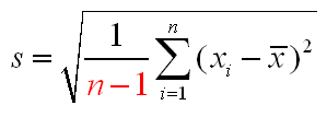
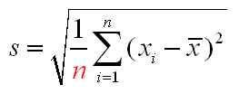
Possibly the most frequently asked and least frequently answered question is why does the definition of the standard deviation involve division by n-1, when n might seem the obvious choice. This is a question which perplexes introductory statistics students and calculator manufacturers alike. The explanations given in calculator manuals tend to range from obscure to fanciful, and both options are given on the keypad, usually labelled sn–1 and sn to add to the confusion. (The symbol s is reserved for the standard deviation of a random variable or a population/distribution, an entity which lecturers valiantly try but usually fail to keep distinct from its sample counterpart.) Australian students first meet the standard deviation in secondary school, where the definition given does indeed involve division by n. This definition is preferred to avoid the question about the n-1 being raised it would seem. Secondary school teachers have a hard enough life as it is. And it must be remembered that the difference between the two definitions is largely academic for all but the smallest of sample sizes (say, less than 10 observations). So, don’t get too agitated by the revamped definition. The truth can be told but the telling usually quells the desire to know. If the fire still burns in your belly, read on.
The most widely accepted explanation involves the concept of unbiasedness, and I see some have stopped reading already. If you fire arrows at a target and consistently hit a mark 5 cm to the left of the bullseye, there is something wrong with your aim. It shows a bias. The definition of the sample variance which involves division by n has this flaw. It consistently underestimates the variance of the population/distribution from which the sample was drawn. The n-1 formula fixes the astigmatism. Compelling and relatively simple as this argument is, it doesn’t quite ring true. Both definitions of the sample standard deviation produce biased estimates of the standard deviation of the population/distribution, although the n-1 alternative is less biased. If you’re after unbiasedness, why not use a definition which gives you unbiasedness where it’s needed – on the original scale of measurement, rather than on the squared scale. Such a contender exists, but it involves gamma functions in the definition, and I see quite a few more people have drifted away. (Gamma functions extend the concept of factorials to non-integers.)
The real reason is a simple housekeeping issue. If you deal with the n-1 straight away in the definition of the standard deviation, it doesn’t keep popping up in every subsequent procedure involving the standard deviation, to the increasing annoyance of all concerned. The subsequent procedures in question involve the definition of the t and c2 distributions where the issue of degrees of freedom arises. Degrees of freedom means what it says – in how many independent directions can you move at once. If you’re a point moving on a page, you are moving in two dimensions and you have correspondingly two degrees of freedom. The freedom to move up the page and the freedom to move across it. Any motion on a page can be described in terms of these two independent motions. Now consider a sample of size n. It inhabits an n dimensional space. There are n degrees of freedom in total. Each sample member is free to take any value it likes, independently from all the others. If however, you fix the sample mean, then the sample values are constrained to have a fixed sum. You can let n-1 of them roam free, but the value of the remaining sample value is determined by the fixed sum. The space inhabited by the deviations from the sample mean is thus n-1 dimensional rather than n dimensional, since the deviations must sum to zero. The sum of the squared deviations, although looking like a sum of n things is actually a sum of only n-1 independent things, and its natural divisor – its degrees of freedom – is also n-1.
But wait, there’s more. Degrees of freedom will return to haunt you if and when you do analysis of variance (ANOVA to its friends). You will be ahead of the game if you grasp the concept now. Degrees of freedom can neither be created nor destroyed. You start off with n, the sample size. You use up a few trying to estimate the structure of the mean. For example, the mean could be a straight line, as in simple linear regression. You need two degrees of freedom to estimate the two characteristics possessed by all straight lines – a slope and an intercept. These characteristics are called parameters. So, two degrees of freedom have gone into the mean. This is the signal. Everything else in this model is noise. The remaining n-2 degrees of freedom go into estimating the one parameter which describes the noise – the variance. If you’re not part of the solution (the signal or mean) you’re part of the problem (the noise). The simplest model is the one which says the mean is a single constant, ably estimated by the sample mean. Everything else is just inexplicable variation about that constant. That’s n-1 degrees of freedom’s worth of noise, all kindly donated to the sample variance.
“I think we’re on the road to coming up with answers that I don’t think any of us in total feel we have the answers to. Kim Anderson, mayor of Naples, Florida”
“Many attempts to communicate are nullified by saying too much.” —in Servant Leadership by Robert Greenleaf

链接已加上,常联系,你的文章很专业
hehe 我来咯
`连blog也跟着人一起牛逼起来了~!
i think n-1 is for sample mean in Statistic
n is for population mean in Statistc
this problem is much popular in Statistic. because everyone will ask that the standard deviation is much different if you are the firt time to study Statistic when you divided by n-1 rather than n. If you want to find the reason, you can check the book named Introduction To the Practice Of Statistics (David s.moore & George p.maccabe)
ya, that's our textbook.
If you want to read a reader’s feedback , I rate this article for 4/5. Detailed info, but I have to go to that damn yahoo to find the missed parts. Thank you, anyway!
Excellent article
have been finding ans for same for 5 years
thnx for meticulous n crisp explanation
Many thanks for the clear explanation. And thanks to Google as well since I found this article by searching with the string “why-divide-by-n-1-and-not-n”.
Cheers from Italy.
Lorenzo
great detailed answer. thank you!
This is not helpful… tomuch bla bla bla nad nothing at the end…. thanks anyway for taking my time
The best answer to the question I’ve seen so far. Now, if only it could be shrunk down to one short and simple sentence.
Nice answer … I’ve ask that question myself. Thanks.